W . Now, we can determine the coefficient of an edge (variable) in constant
time.
W . Now, we can determine the coefficient of an edge (variable) in constant
time.
In this section we describe the different subtrees in the class hierarchy and their classes. We give this description not in the form of a manual by describing each member of the class (this is later done partially in Chapter 5 and in detail in the reference manual), but we try to explain the problems, our ideas, why we designed the class hierarchy and the single classes as we did, and discuss also some alternatives.
It is well known that global variables, constants, or functions can cause a lot of problems within a big software system. This is even worse for frameworks such as ABACUS that are used by other programmers and may be linked together with other libraries. Here, name conflicts and undesired side effects are almost inevitable. Since global variables can also make a future parallelization more difficult we have avoided them completely.
We have embedded functions and enumerations that might be used by all other classes in the class ABA_ABACUSROOT. We use this class as a base class for all classes within our systems. Since the class ABA_ABACUSROOT contains no data members, objects of derived classes are not blown up.
Currently, ABA_ABACUSROOT implements only an enumeration with the different exit codes of the framework and implements some public member functions. The most important one of them is the function exit(), which calls the system function exit(). This construction turns out to be very helpful for debugging purposes.
In an object oriented implementation of a linear-programming based branch-and-bound algorithm we require one object that controls the optimization, in particular the enumeration and resource limits, and stores data that can be accessed from any other object involved in the optimization of a specific instance. This task is performed by the class ABA_MASTER, which is not identical with the root node of the enumeration tree. For each application of ABACUS we have to derive a class from ABA_MASTER implementing problem specific “global” data and functions.
Every object, which requires access to this “global” information, stores a pointer to the corresponding object of the class ABA_MASTER. This holds for almost all classes of the framework. For example the class ABA_SUB, implementing a subproblem of the branch-and-bound tree, has as a member a pointer to an object of the class ABA_MASTER (other members of the class ABA_SUB are omitted):
class ABA_SUB {
ABA_MASTER *master_; }; |
Then, we can access within a member function of the class ABA_SUB, e.g., the global upper bound by calling
master_->upperBound();
|
where upperBound() is a member function of the class ABA_MASTER.
Encapsulating this global information in a class is also important, if more than one linear-programming based branch-and-bound is solved within one application. If the pricing problem within a branch-and-price algorithm is again solved with the help of ABACUS, e.g., then separate master objects with different global data are used.
Within a specific application there are always some global data members as the output and error streams, zero tolerances, a big number representing “infinity”, and some functions related with these data. For the same reasons we discussed already in the description of the class ABA_ABACUSROOT we should avoid storing these data in global variables. It is also not reasonable to add these data to the class ABA_ABACUSROOT, because it would blow up every derived class of ABA_ABACUSROOT and it is neither necessary nor desired to have extra output streams, zero tolerances, etc., for every object.
Instead of implementing this data directly in the class ABA_MASTER we designed an extra class ABA_GLOBAL, from which the class ABA_MASTER is derived. The reason is that there are several classes, especially some basic data structures, which might be useful in programs that are not branch-and-bound algorithms. To simplify their reuse these classes have a pointer to an object of the class ABA_GLOBAL instead of one to an object of the class ABA_MASTER.
The class ABA_MASTER augments the data inherited from the class ABA_GLOBAL with specific data members and functions for branch-and-bound. It has objects of classes as members that store the list of subproblems which still have to be processed in the implicit enumeration (class ABA_OPENSUB), and that store the variables which might be fixed by reduced cost criteria in later iterations (class ABA_FIXCAND). Moreover, the solution history, timers for parts of the optimization, and a lot of other statistical information is stored within the class ABA_MASTER.
The class ABA_MASTER also provides default implementations of pools for the storage of constraints and variables. We explain the details in Section 4.2.5.
A branch-and-bound framework requires also a flexible way for defining enumeration strategies. The corresponding virtual functions are defined in the class ABA_MASTER, but for a better understanding we explain this concept in Section 4.2.7, when we discuss the data structure for the open subproblems.
The control of limits on the optimization process, e.g., the amounts of CPU time and wall-clock time, and the size of the enumeration tree are performed by members of the class ABA_MASTER during the optimization process. Also the guarantee of the solution is monitored by the class ABA_MASTER.
When the optimization is started, the root node of the branch-and-bound tree has to be initialized with an object of the class ABA_SUB. However, the class ABA_SUB is an abstract class, from which a class implementing the problem specific features of the subproblem optimization has to be derived. Therefore, the initialization of the root node is performed by a pure virtual function returning a pointer to a class derived from the class ABA_SUB. This function has to be defined by a problem specific class derived from the class ABA_MASTER.
For simplification often programs that can be used for minimization and maximization problems use internally only one sense of the optimization, e.g., maximization. Within a framework this strategy is dangerous, because if we access internal results, e.g., the reduced costs, from an application, we might misinterpret them. Therefore, ABACUS also works internally with the true sense of optimization. The value of the best known feasible solution is denoted primal bound, the value of a linear programming relaxation is denoted dual bound if all variables price out correctly. The functions lowerBound() and upperBound() interpret the primal or dual bound, respectively, depending on the sense of the optimization. An equivalent method is also used for the local bounds of the subproblems.
Computer programs in a UNIX environment often use configuration files for the control of certain parameters. Usually, these parameters are stored in the home directory of the user or the directory of the program and start with a ‘.’. We use a similar concept for reading the parameters of ABACUS. These parameters are read from the file .abacus.
However, as ABACUS is a framework for the implementation of different algorithms, there are further requirements for the parameter concept. First, there should be a simple way for reading problem specific parameters. An extendable parameter format should relieve the user of opening and reading his own parameter files. Second, a user of our system might have several applications. It should be possible to specify parameters for different applications and to redefine application dependent parameters defined in the file .abacus.
Therefore, we provide the following parameter concept. All parameters read from the file .abacus are written into a dictionary. Application specific parameters can be specified in extra parameter files following a very simple format. For files using our parameter format we provide already an input function. The parameters read by this input function are also written to the parameter dictionary. Hence, parameters of the file .abacus can be easily redefined. Moreover, we also provide simple functions to extract the values of the parameters from the dictionary.
The parameters in .abacus include limits on the resources of the optimization process, control of various strategies (e.g., the enumeration strategy, the branching strategy, zero tolerances for various decisions, the amount of output, parameters for the LP-solver). A detailed list of parameters can be found in Section 5.2.26.
The class ABA_SUB represents a subproblem of the implicit enumeration, i.e., a node of the branch-and-bound tree. The class subproblem is an abstract class, from which a problem specific subproblem has to be derived. In this derivation process problem specific functions can be added, e.g., for the generation of variables or constraints.
For the root node of the optimization the constraint and variable sets can be initialized explicitly. As in many applications the initial variable and constraint sets are in a one-to-one correspondence with the items of the initial variable and constraint pools, we provide this default initialization mechanism. By default, the first linear program is solved with the barrier method followed by a crossover to a basic solution, but we provide a flexible mechanism for the selection of the LP-method (see Section 5.2.11).
As long as only globally valid constraints and variables are used it would be correct to initialize the constraint and variable system of a subproblem with the system of the previously processed subproblem. However, ABACUS is designed also for locally valid constraints and variables. Therefore, each subproblem inherits the final constraint and variable system of the father node in the enumeration tree. This system might be modified by the applied branching rule. Moreover, this approach avoids also tedious recomputations and makes sure that heuristically generated constraints do not get lost.
If conventional branching strategies, like setting a binary variable, changing the bounds of an integer variable, or even adding a branching constraint are applied, then the basis of the last solved linear program of the father is still dual feasible. As we store the basis status of the variables and slack variables we can avoid phase 1 of the simplex method if we use the dual simplex method.
If due to another branching method, e.g., for branch-and-price algorithms, the dual feasibility of the basis is lost, another LP-method can be used.
A linear-programming based branch-and-bound algorithm in its simpliest form is obtained if linear programming relaxations in each subproblem are solved that are neither enhanced by the generation of cutting planes nor by the dynamic generation of variables. Such an algorithm requires only two problem specific functions: one to check if a given LP-solution is a feasible solution of the optimization problem, and one for the generation of the sons.
The first function is problem specific, because, if constraints of the integer programming formulation are violated, the condition that all discrete variables have integer values is not sufficient. Therefore, for safety this function is declared pure virtual.
The second required problem specific function is usually only a one-liner, which returns the problem specific subproblem generated by a branching rule.
Hence, the implementation of a pure branch-and-bound algorithm does not require very much effort.
The core of the class ABA_SUB is its optimization by a cutting plane algorithm. As dynamically generated variables are dual cuts we also use the notion cutting plane algorithm for a column generation algorithm. By default, the cutting plane algorithm only solves the LP-relaxation and tries to fix and set variables by reduced costs. Within the cutting plane algorithm four virtual dummy functions for the separation of constraints, for the pricing of variables, for the application of primal heuristics, and for fixing variables by logical implications are called. In a problem specific class derived from the class ABA_SUB these virtual functions can be redefined. Motivated by duality theory (see [Thi95]), we handle constraint and variable generation equivalently. If both constraints and variables are generated, then by default constraints are generated. In addition to the mandatory pricing phase before the fathoming of a subproblem, we price out the inactive variables every k iterations. The value of k can be controlled by a parameter. By the redefinition of a virtual function other strategies for the separation/pricing decision can be implemented.
Cutting planes may not only be generated in the function separate() but also in other functions of the cutting plane phase. For the maximum cut problem, e.g., it is advantageous if the generation of cutting planes is also possible in the function improve(), in which usually primally feasible solutions are computed heuristically. If not all constraints of the integer programming formulation are active, then it might be necessary to solve a separation problem also for the feasibility test. Therefore, we allow the generation of cutting planes in every subroutine of the cutting plane algorithm.
Like for constraints, we also allow the generation of variables during the complete subproblem optimization.
New constraints and variables are not immediately added to the subproblem, but stored in buffers and added at the beginning of the next iteration. We present the details of this concept in Section 4.2.7.
In order to avoid corrupting the linear program and the sets of active constraints and variables, and to allow the removal of variables and constraints in any subroutine of the cutting plane phase, we also buffer these variables and constraints. The removal is executed before constraints and variables are added at the beginning of the next iteration of the cutting plane algorithm.
Moreover, we provide default functions for the removal of constraints according to the value or the basis status of the slack variables. Variables can be removed according to the value of the reduced costs. These operations can be controlled by parameters and the corresponding virtual functions can be redefined if other criteria should be applied. We try to remove constraints also before a branching step is performed.
In order to allow a flexible combination of constraint and variable generation, every subproblem has its own set of active constraints and variables, which are represented by the generic class ABA_ACTIVE. By default, the variables and the constraints of the last solved linear program of the father of the subproblem are inherited. Therefore, the local constraint and variable sets speed up the optimization. The disadvantage of these local copies is that more memory is allocated per subproblem. However, this local storage of the active constraints and variables will simplify a future parallelization of the framework.
Together with the active constraints and variables we also store in every subproblem the LP-statuses of the variables and slack variables, the upper and lower bounds of the variables, and if a variable is fixed or set.
As for active constraints and variables also every subproblem has its own linear program, which is only set up for an active subproblem. Of course, the initialization at the beginning and the deletion of the linear program at the end of the subproblem optimization costs some running time compared to a global linear program, which could be stored in the master. However, a local linear program in every subproblem will again simplify the implementation of a parallel version of ABACUS. Our current computational experience shows that this overhead is not too big. However, if in future computational experiments it turns out that these local linear programs slow down the overall running time significantly, the implementation of a special sequential version of the code with one global linear program will not be too difficult, whereas the opposite direction would be harder to realize.
Currently, three different methods are available in state-of-the-art LP-solvers: the primal simplex method, the dual simplex method, and the barrier method in combination with crossing over techniques for the determination of an optimal basic solution. The choice of the method can be essential for the performance of solution of the linear program. If a primal feasible basis is available, the primal simplex method is often the right choice. If a dual feasible basis is available, the dual simplex method is usually preferred. And finally, if no basis is known, or the linear programs are very large, often the barrier methods yields the best running times.
Currently the Open Solver Interface used by ABACUS does not support the barrier method. Nevertheless a barrier method is provided for compatibility to older versions of ABACUSṪhis method outputs a warning message and calls the primal simplex method. By default a linear program is solved by the primal simplex method, and by the dual simplex method, if constraints have been added, or variables have been removed, or it is the first linear program of a subproblem.
However, it should be possible to add problem specific decision criteria. Here, again a virtual function gives us all flexibility. We keep control when this function is invoked, namely at the point when all decisions concerning addition and removal of constraints and variables have been taken. The function has as arguments the correct numbers of added and removed constraints and variables. If we want to choose the LP-method problem specifically, then we only have to redefine this function in a class derived from the class ABA_SUB.
If constraint and variable generation are combined, then the active constraints must be lifted if a variable is added, i.e., the column of the new variable must be computed. This lifting can not always be done in a straightforward way, it can even require the solution of another optimization problem. Moreover, lifting is not only required when a variable is added, but this problem has to be attacked already during the solution of the pricing problem.
In order to allow the usage of constraints that cannot be lifted or for which the lifting cannot be performed efficiently, we provide a management of non-liftable constraints. Each constraint has a flag if it is liftable. If the pricing routine is called and non-liftable constraints are active, then all non-liftable constraints are removed, the linear programming relaxation is solved again, and we continue with the cutting plane algorithm before we come back to the pricing phase. In order to avoid an infinite repetition of this process we forbid the further generation of non-liftable constraints during the rest of the optimization of this subproblem.
If the root of the remaining branch-and-bound tree changes, but the new root has been processed earlier, then it can be advantageous to optimize the corresponding subproblem again, in order to get improved conditions for fixing variables by reduced costs. Therefore, we provide the reoptimization of a subproblem. The difference to the ordinary optimization is that no branching is finally performed even if the subproblem is not fathomed. If it turns out during the reoptimization that the subproblem is fathomed, then we can fathom all subproblems contained in the subtree rooted at this subproblem.
Virtual functions for the flexible definition of branching strategies are implemented in the class ABA_SUB. We explain them together with the concept of branching rules in Section 4.2.7.
If constraints are generated heuristically, then the concept of delayed branching can be advantageous. Instead of generating the sons of a subproblem in a branching step, the subproblem is put back into the set of open subproblems. There it stays several rounds dormant, i.e., other subproblems are optimized in the meantime, until the subproblem is processed again. If between two successive optimizations of the subproblem good cutting planes are generated that can be separated from the pool, then this technique can accelerate the optimization. The maximal numbers of optimizations and the minimal number of dormant rounds can be controlled by parameters.
Since constraints and variables are added and removed dynamically, we also provide a dynamic memory management system, which requires no user interaction. If there is not enough memory already allocated to add a constraint or variable, memory reallocations are performed automatically. As the reallocation of the local data, in particular of the linear program, can require a lot of CPU time, if it is performed regularly, we allocate some extra space for the addition of variables and constraints, and for the nonzero entries of the matrix of the LP-solver.
In order to save memory we set up those data structures that are only required if the subproblem is active, e.g., the linear program, at the beginning of the subproblem optimization and delete the memory again when the subproblem becomes inactive. We observed that the additional CPU time required for these operations is negligible, but the memory savings are significant.
Constraints and variables are central items within linear-programming based branch-and-bound algorithms. As ABACUS is a system for general mixed integer optimization problems and combinatorial optimization problems we require an abstract concept for the representation of constraints and variables. Linear programming duality motivated us to embed common features of constraints and variables in a joint base class.
Usually, the notions constraint and row, and the notions variable and column, respectively, are used equivalently.
Within ABACUS constraints and rows are different items. Constraints are stored in the pool and a subproblem has a set of active constraints. Only if a constraint is added to the linear program, then the corresponding row is computed. More precisely, a row is a representation of a constraint associated with a certain variable set.
The reasons for this differentiation can be explained with the subtour elimination constraints of the traveling salesman problem, which are defined for subsets W of the nodes of a graph as x(E(W)) ≤|W|- 1. Storing this inequality as it is added to the linear program would require to store all edges (variables) with both endnodes in the set W . Such a format would require O(|W|2) storage space. However, it would be also sufficient to store the node set W requiring 0(|W|) storage space. Given the variable e associated with the edge (t,h), then the coefficient of e in the subtour elimination constraint is 1 if t and h are contained in W , 0 otherwise.
For the solution of the traveling salesman problem we also want to apply sparse graph techniques. Therefore, storing the coefficients of all active and inactive variables of a subtour elimination constraint would waste a lot of memory. If we store only the coefficients of the variables that are active when the constraint is generated, then the computation of the coefficient of an added variable would be difficult or even impossible. However, if we store all nodes defining the constraint, then the coefficients of variables that are later added can be determined easily.
Efficient memory management and dynamic variable generation are the reason why we distinguish between constraints and rows. Each constraint must have a member function that returns the coefficient for a variable such that we can determine the row corresponding to a set of variables.
In these considerations “constraint” can be also replaced by “variable” and “row” by “column”. A column is the representation of a variable corresponding to a certain constraint set. Again, we use the traveling salesman problem as example. A variable for the traveling salesman problem corresponds to an edge in a graph. Hence, it can be represented by its end nodes. The column associated with this variable consists of the coefficients of the edge for all active constraints.
We implemented these concepts in the classes ABA_CONSTRAINT/ABA_VARIABLE, which are used for the representation of active constraints and variables and for the storage of constraints and variables in the pools, and ABA_ROW/ABA_COLUMN, which are used in particular in the interface to the LP-solver.
This differentiation between constraints/variables and rows/columns is not used by any other system for the implementation of linear-programming based branch-and-bound algorithms, because they are usually designed for the solution of general mixed integer optimization problems, which do not necessarily require this distinction. However, this concept is crucial for a practically efficient and simple application of ABACUS to combinatorial optimization problems.
Constraints and variables have several common features, which we consider in a common base class.
A constraint/variable is active if it belongs to the constraint/variable set of an active subproblem. An active constraint/variable must not be removed from its pool. As in a parallel implementation of ABACUS there can be several active subproblems, each constraint/variable has a counter for the number of active subproblems, in which it is active.
Besides being active there can be other reasons why a constraint/variable should not be deleted from its pool, e.g., if the constraint/variable has just been generated, then it is put into a buffer, but is not yet activated (we explain the details in Section 4.2.7). In such a case we want to set a lock on the constraint that it cannot be removed. Again, in a parallel implementation, but also in a sequential one, we may want to set locks at the same time on the same constraint for different reasons. Hence, we count the number of locks of each constraint/variable.
Constraints and variables can be locally or globally valid. Therefore, we provide a flag in the common base class of constraints and variables. The functions to determine if a local constraint or variable is valid for a certain subproblem are associated directly with the classes for constraints and variables, respectively.
It has been stated that the use of locally valid constraints and variables should be avoided as it requires a nasty bookkeeping [PR91]. In order to free the user from this, we have embedded the management of local constraints and variables in ABACUS. The validity of a constraint/variable is automatically checked if it is regenerated from the pool.
We also distinguish between dynamic variables/constraints and static ones. As soon as a static variable/constraint becomes active it cannot be deactivated. An example for static variables are the variables in a general mixed integer optimization problem, examples for static constraints are the constraints of the problem formulation of a general mixed integer optimization problem or the degree constraints of the traveling salesman problem. Dynamic constraints are usually cutting planes. In column generation algorithm variables can be dynamic, too.
A crucial point in the implementation of a special variable or constraint class is the tradeoff between performance and memory usage. We have observed that a memory efficient storage format can be one of the keys to the solutions of larger instances. Such formats are in general not very useful for the computation of the coefficient of a single variable/constraint. Moreover, if the coefficients of a constraint for several variables or the coefficients of a variable for several constraints have to be computed, e.g., when the row/column format of the constraint/variable is generated in order to add it to the LP-solver, then these operations can become a bottleneck. However, given a different format, using more memory, it might be possible to perform these operations more efficiently.
Therefore, we distinguish between the compressed format and the expanded format of a constraint/variable. Before a bigger number of time consuming coefficient computations is performed, we try to generate the expanded format, afterwards the constraint/variable is compressed.
Of course, both expanded and compressed formats are rather constraint/variable specific. But we provide the bookkeeping already in the common base class and try to expand the constraint/variable, e.g., when it is added to the linear program. Afterwards it is compressed again. The implementation of the expansion and compression is optional.
We use again the subtour elimination constraint of the traveling salesman problem as an example for the compressed and
expanded format. For an inequality x(E(W)) ≤|W|- 1 we store the nodes of the set W in the compressed
format. The computation of the coefficient of an edge (t,h) requires O(|W|) time and space. As expanded
format we use an array inSubtour of type bool of length n (n is the number of nodes of the graph) and
inSubtour[v] is true if and only if v W . Now, we can determine the coefficient of an edge (variable) in constant
time.
ABACUS provides all three different types of constraints: equations, ≤-inequalities and ≥-inequalities. The only pure virtual function is the computation of a coefficient of a variable. We use this function to generate the row format of a constraint, to compute the slack of an LP-solution, and to check if an LP-solution violates a constraint. All these functions are declared virtual such that they can be redefined for performance reasons.
We distinguish between locally and globally valid constraints. By default, a locally valid constraint is considered to be valid for the subproblem it was generated and for all subproblems in the tree rooted at this subproblem. This criterion is implemented in a virtual function such that it can be redefined for special constraints.
If variables are generated dynamically, we distinguish between liftable and non-liftable constraints. Non-liftable constraints have to be removed before the pricing problem can be solved (see Section 4.2.3).
ABACUS provides a default non-abstract constraint class with the class ABA_ROWCON, where a constraint is represented by its row format, i.e., only the numbers of variables with nonzero coefficients and the corresponding coefficients are stored. This format is useful, e.g., for constraints of general mixed integer optimization problems. From the class ABA_ROWCON we derive the class ABA_SROWOCN, which implements some member functions more efficiently as it assumes that the variable set is static, i.e., no variables are generated dynamically.
ABACUS supports continuous, integer, and binary variables in the class ABA_VARIABLE. Each variable has a lower and an upper bound, which can be set to plus/minus infinity if the variable is unbounded. We also memorize if a variable is fixed.
The following functions have their dual analogons in the class ABA_CONSTRAINT. The only pure virtual function is now the function that returns a coefficient in a constraint. With this function the generation of the column format and the computation of the reduced cost can be performed. We say a variable is violated if it does not price out correctly.
Also variables can be locally or globally valid. A subproblem is by default associated with a locally valid variable. The variable is then valid in all subproblems on the path from this subproblem to the root node. Of course, this virtual function can be redefined for problem specific variables.
We provide already a non-abstract derived variable class. The class ABA_COLVAR implements a variable that is represented by the column format, i.e., only the nonzero coefficients together with the numbers of the corresponding rows are stored.
Every constraint and variable either induced by the problem formulation or generated in a separation or pricing step is stored in a pool. A pool is a collection of constraints and variables. We will see later that it is advantageous to keep separate pools for variables and constraints. Then, we will also discuss when it is useful to have also different pools for different types of constraints or variables. But for simplicity we assume now that there is only one variable pool and one constraint pool.
There are two reasons for the usage of pools: saving memory and an additional separation/pricing method.
A constraint or variable usually belongs to the set of active constraints or variables of several subproblems that still have to be processed. Hence, it is advantageous to store in the sets of active constraints or variables only pointers to each constraint or variable, which is stored at some central place, i.e., in a pool that is a member of the corresponding master of the optimization. Our practical experiments show that this memory sensitive storage format is of very high importance, since already this pool format uses a large amount of memory.
From the point of view of a single subproblem a pool may not only contain active but also inactive constraints or variables. The inactive items can be checked in the separation or pricing phase, respectively. We call these techniques pool separation and pool pricing. Again, motivated by duality theory we use the notion “separation” also for the generation of variables, i.e., for pricing. Pool separation is advantageous in two cases. First, pool separation might be faster than the direct generation of violated constraints or variables. In this case, we usually check the pool for violated constraints or variables, and only if no item is generated, we use the more time consuming direct method. Second, pool separation turns out to be advantageous, if a class of constraints or variables can be separated/priced out only heuristically. In this case, it can happen that the heuristic cannot generate the constraint or variable although it is violated. However, earlier in the optimization process this constraint or variable might have been generated. In this case the constraint or variable can be easily regenerated from the pool. Computational experiments show that this additional separation or pricing method can decrease the running time significantly [JRT94].
During the regeneration of constraints and variables from the pools we also have to take into account that a constraint or variable might be only locally valid.
The pool separation is also one reason for using different pools for variables and constraints. Otherwise, each item would require an additional flag and a lot of unnecessary work would have to be performed during the pool separation.
Pool separation is also one of the reasons why it can be advantageous to provide several constraint or variable pools. Some constraints, e.g., might be more important during the pool separation than other constraints. In this case, we might check this “important” pool first and only if we fail in generating any item we might proceed with other pools or continue immediately with direct separation techniques.
Other classes of constraints or variables might be less important in the sense that they cannot or can only very seldomly be regenerated from the pool (e.g., locally valid constraints or variables). Such items could be kept in a pool that immediately removes all items that do not belong to the active constraint or variable set of any subproblem which still has to be processed. A similar strategy might be required for constraints or variables requiring a big amount of memory.
Finally, there are constraints for which it is advantageous to stay active in any case (e.g., the constraints of the problem formulation in a general mixed integer optimization problem, or the degree constraints for the traveling salesman problem). Also for these constraints separate pools are advantageous.
In any case, as soon as a lot of constraints or variables are generated dynamically we can observe that the pools become very, very large. In the worst case this might cause an abnormal termination of the program if it runs out of memory. But already earlier the optimization process might be slowed down since pool separation takes too long. Of course, the second point can be avoided by limited strategies in pool separation, which we will discuss later. But to avoid the first problem we require suitable cleaning up and garbage collection strategies.
The simplest strategy is to remove all items belonging not to any active variable or constraint set of any active or open subproblem in a garbage collection process. The disadvantage of this strategy might be that good items are removed that are accidentally momentarily inactive. A more sophisticated strategy might be counting the number of linear programs or subproblems where this item has been active and removing initially only items with a small counter.
Unfortunately, if the enumeration tree grows very large or if the number of constraints and variables that are active at a single subproblem is high, then even the above brute force technique for the reduction of a pool turns out to be insufficient.
Hence, we have to divide constraints and variables into two groups. On the one hand the items that must not be removed from the pool, e.g., the constraints and variables of the problem formulation of a general mixed integer optimization problem, and on the other hand those items that can either be regenerated in the pricing or separation phase or are not important for the correctness of the algorithm, e.g., cutting planes. If we use the data structures we will describe now, then we can remove safely an item of the second group.
So far, we have assumed that the sets of active variables or constraints store pointers to variables or constraints, respectively, which are stored in pools. If we would remove the variable or constraint, i.e., delete the memory we have allocated for this object, then errors can occur if we access the removed item from a subproblem. These fatal errors could be avoided if a message is sent to every subproblem where the deleted item is currently active. This technique would require additional memory and running time. Therefore, we propose a data structure that can handle this problem very simply and efficiently.
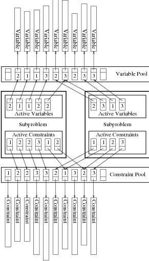
A pool is not a collection of constraints or variables, but a collection of pool slots (class ABA_POOLSLOT). Each slot stores a pointer to a constraint or variable or a 0-pointer if it is void. The sets of active constraints or variables store pointers to the corresponding slots instead of storing pointers to the constraints or variables directly. So, if a constraint or variable has been removed a 0-pointer will be found in the slot and the subproblem recognizes that the constraint or variable must be eliminated since it cannot be regenerated. The disadvantage of this method is that finally our program may run out of memory since there are many useless slots.
In order to avoid this problem we add a version number as data member to each pool slot. Initially the version number is 0 and becomes 1 if a constraint or variable is inserted in the slot. After an item in a slot is deleted a new item can be inserted into the slot. Each time a new item is stored in the slot the version number is incremented. The sets of active constraints and variables do not only store pointers to the corresponding slots but also the version number of the slot when the pointer is initialized. If a member of the active constraints or variables is accessed we compare its original and current version number. If these numbers are not equal we know that this is not the constraint or variable we were originally pointing to and remove it from the active set. We call the data structure storing the pointer to the pool slot and the original version number a reference to a pool slot (class ABA_POOLSLOTREF). Hence, the sets of active constraints and variables are arrays of references to pool slots. We present an example for this pool concept in Figure 4.1. The numbers in the boxes are arbitraryly chosen version numbers.
The class ABA_POOL is an abstract class, which does not specify the storage format of the collection of pool slots. The simplest implementation is an array of pool slots. The set of free pool slots can be implemented by a linked list. This concept is realized in the class ABA_STANDARDPOOL. Moreover, a ABA_STANDARDPOOL can be static or dynamic. A dynamic ABA_STANDARDPOOL is automatically enlarged, when it is full, an item is inserted, and the cleaning up procedure fails. A static ABA_STANDARDPOOL has a fixed size and no automatic reallocation is performed.
More sophisticated implementations might keep an order of the pool slots such that “important” items are detected earlier in a pool separation such that a limited pool separation might be sufficient. A criterion for this order could be the number of subproblems where this constraint or variable is active or has been active. We will consider such a pool in a future release.
The number of the pools is very problem specific and depends mainly on the separation and pricing methods. Since in many applications a pool for variables, a pool for the constraints of the problem formulation, and a pool for cutting planes are sufficient, we implemented this default concept. If not specified differently, in the initialization of the pools, in the addition of variables and constraints, and in the pool pricing and pool separation these default pools are used. We use a static ABA_STANDARDPOOL for the default constraint and cutting planes pools. The default variable pool is a dynamic ABA_STANDARDPOOL, because the correctness of the algorithm requires that a variable which does not price out correctly can be added in any case, whereas the loss of a cutting plane that cannot be added due to a full pool has no effect on the correctness of the algorithm as long as it does not belong to the integer programming formulation.
If instead of the default pool concept an application specific pool concept is implemented, then the user of the framework must make sure that there is at least one variable pool and one constraint pool and these pools are embedded in a class derived from the class ABA_MASTER.
With this concept we provide a high flexibility: An easy to use default implementation, which can be changed by the redefinition of virtual functions and the application of non-default function arguments.
All classes involved in this pool concept are designed as generic classes such that they can be used both for variables and constraints.
Since ABACUS is a framework for the implementation of linear-programming based branch-and-bound algorithms it is obvious that the solution of linear programs plays a central role, and we require a class concept of the representation of linear programs. Moreover, linear programs might not only be used for the solution of LP-relaxations in the subproblems, but they can also be used for other purposes, e.g., for the separation of lift-and-project cutting planes of zero-one optimization problems [BCC93a, BCC93b] and within heuristics for the determination of good feasible solutions in mixed integer programming [HP93].
Therefore, we would like to provide two basic interfaces for a linear program. The first one should be in a very general form for linear programs defined by a constraint matrix stored in some sparse format. The second one should be designed for the solution of the LP-relaxations in the subproblem. The main differences to the first interface are that the constraint matrix is stored in the abstract ABA_VARIABLE/ABA_CONSTRAINT format instead of the ABA_COLUMN/ABA_ROW format and that fixed and set variables should be eliminated.
Another important design criterion is that the solution of the linear programs should be independent from the used LP-solver, and plugging in a new LP-solver should be simple.
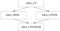
The result of these requirements is the class hierarchy of Figure 4.2. The class ABA_LP is an abstract base class providing the public functions that are usually expected: initialization, optimization, addition of rows and columns, deletion of rows and columns, access to the problem data, the solution, the slack variables, the reduced costs, and the dual variables. These functions do some minor bookkeeping and call a pure virtual function having the same name but starting with an underscore (e.g, optimize() calls _optimize). These functions starting with an underscore are exactly the functions that have to be implemented by an interface to an LP-solver.
The class ABA_OSIIF implements these solver specific functions. The class ABA_OSIIF itself is an interface to Osi (Open Solver Interface) which is a uniform API for calling embedded linear and mixed-integer programming solvers. Using this generic API means that the single interface class ABA_OSIIF provides access to a whole range of LP-solvers. Another advantage is that any change in the API of a specific LP-solver is handled by th Osi layer. That means that in order to support future versions of LP-solvers no change to the ABACUS code will be necessary. When support for futher solvers is added to Osi only minimal changes to ABACUS will be necessary to make them available for solving linear programs.
The most important linear programs being solved within this system are the LP-relaxations solved in the optimization of the subproblems. However, the active constraints and variables of a subproblem are not stored in the format required by the class ABA_LP. Therefore, we have to implement a transformation from the ABA_VARIABLE/ABA_CONSTRAINT format to the ABA_COLUMN/ABA_ROW format.
Two options are available for the realization of this transformation: either it can be implemented in the class ABA_SUB or in a new class derived from the class ABA_LP. We decided to implement such an interface class, which we call ABA_LPSUB, for the following reasons. First, the interface is better structured. Second, the subproblem optimization becomes more robust for later modifications of the class ABA_LP. Third, we regard the class ABA_LPSUB as a preprocessor for the linear programs solved in the subproblem, because fixed and set variables can be eliminated from the linear program submitted to the solver. It depends on the used solution method if all fixed and set variables should be eliminated. If the simplex method is used and a basis is known, then only nonbasic fixed and set variables should be eliminated. The encapsulation of the interface between the subproblem and the class ABA_LP supports a more flexible adaption of the elimination to other LP-solvers in the future and also enables us to use other LP-preprocessing techniques, e.g., constraint elimination, or changing the bounds of variables under certain conditions (see [Sav94]), without modifying the variables and constraints in the subproblem. Preprocessing techniques other than elimination of fixed and set variables are currently not implemented.
The subproblem optimization in the class ABA_SUB uses only the public functions of the class ABA_LPSUB, which is again an abstract class independent from the used LP-solver.
A linear program solving the relaxations within a subproblem with a LP-solver supported by Osi is defined by the class ABA_LPSUBOSI, which is derived from the classes ABA_LPSUB and ABA_OSIIF. The class ABA_LPSUBOSI only implements a constructor passing the arguments to the base classes. Using a LP-solver not suppported by Osi in this context requires the definition of a class equivalent to the class ABA_LPSUBOSI and a redefinition of the virtual function ABA_LPSUB *ABA_SUB::generateLp(), which is a one-line function allocating an object of the class ABA_LPSUBOSI and returning a pointer to this object.
Therefore, it is easy to use different LP-solvers for different ABACUS applications and it is also possible to use different LP-solvers in a single ABACUS application. For instance, if there is a very fast method for the solution of the linear programs in the root node of the enumeration tree, but all other linear programs should be solved by Cplex, then only a simple modification of ABA_SUB::generateLp() is required.
To avoid multiple instances of the class ABA_LP in objects of the class ABA_LPSUBOSI, the classes ABA_OSIIF, and ABA_LPSUB are virtually derived from the class ABA_LP. In order to save memory we do not make copies of the LP-data in any of the classes of this hierarchy except for the data that is passed to the LP-solvers in the class ABA_OSIIF.
In this section we are going to discuss the design of some important classes that support the linear-programming based branch-and-bound algorithm. These are classes for the management of the open subproblems, for buffering newly generated constraints and variables, for the implementation of branching rules, for the candidates for fixing variables by reduced costs, for the control of the tailing off effect, and for the storage of a solution history.
During a branch-and-bound algorithm subproblems are dynamically generated in branching steps and later optimized. Therefore, we require a data structure that stores pointers to all unprocessed and dormant subproblems and supports the insertion and the extraction of a subproblem.
One of the important issues in a branch-and-bound algorithm is the enumeration strategy, i.e., which subproblem is extracted from the set of open subproblems for further processing. It would be possible to implement the different classical enumeration strategies, like depth-first search, breadth-first search, or best-first search within this class. But in this case, an application-specific enumeration strategy could not be added in a simple way by a user of ABACUS. Of course, with the help of inheritance and virtual functions a technique similar to the one we implemented for the usage of different LP-solvers for the subproblem optimization could be applied. However, there is a much simpler solution for this problem.
In the class ABA_MASTER we define a virtual member function that compares two subproblems according to the selected enumeration strategy and returns 1 if the first subproblem has higher priority, -1 if the second one has higher priority, and 0 if both subproblems have equal priority. Application specific enumeration strategies can be integrated by a redefinition of this virtual function. In order to compare two subproblems within the extraction operation of the class ABA_OPENSUB this comparison function of the associated master is called.
The class ABA_OPENSUB implements the set of open subproblems as a doubly linked linear list. Each time when another subproblem is required for further processing the complete list is scanned and the best subproblem according to the applied enumeration strategy is extracted. This implementation has the additional advantage, that it is very easy to change the enumeration strategy during the optimization process, e.g., to perform a diving strategy, which uses best-first search but performs a limited depth first search every k iterations.
The drawback of this implementation is the linear running time of the extraction of a subproblem. If the set of open subproblems would be implemented by a heap, then the insertion and the extraction of a subproblem would require logarithmic time, whereas in the current implementation the insertion requires constant, but the extraction requires linear time. But if the enumeration strategy is changed, the heap has to be reinitialized from scratch, which requires linear time.
However, it is typical for a linear-programming based branch-and-bound algorithm that a lot of work is performed in the subproblem optimization, but the total number of subproblems is comparatively small. Also the performance analysis of our current applications shows that the running time spent in the management of the set of open subproblems is negligible. Due to the encapsulation of the management of the set of open subproblem in the private part of the class ABA_OPENSUB, it will be no problem to change the implementation, as soon as it is required.
In order to allow the special fathoming technique for fathoming more than one subproblem in case of a contradiction (even though it is currently not implemented), the class ABA_OPENSUB supports also the removal of an arbitrary subproblem. This operation cannot be performed in logarithmic time in a heap, but requires linear time. A data structure providing logarithmic running time for the insertion, extraction of the minimal element, and removal of an arbitrary element is, e.g., a red-black tree [Bay72, GS78]. According to our current experience it seems that the implementation effort for these enhanced data structures does not pay.
We provide four rather common enumeration strategies per default: best-first search, breadth-first search, depth-first search, and a simple diving strategy performing depth-first search until the first feasible solution is found and continuing afterwards with best-first search.
If the branching strategy is branching on a binary variable, then these default enumeration strategies are further refined. We can often observe in mixed integer programming that feasible solutions are sparse, i.e., only a small number of variables have a nonzero value. Setting a binary variable to one may induce a subproblem with a smaller number of feasible solutions than for its brother in which the branching variable is set to zero. Therefore, if two subproblems have the same priority in the enumeration, we prefer that one with the branching variable set to one. This resolution of subproblems having equal priority is performed in a virtual function, such that it can be adapted to each specific application or can be extended to other branching strategies.
Usually, new constraints are generated in the separation phase. However, it is possible that in some applications violated constraints are also generated in other subroutines of the cutting plane algorithm. In particular, if not all constraints of the integer programming formulation are active in the subproblem a separation routine might have to be called to check the feasibility of the LP-solution. Another example is the maximum cut problem, for which it is rather convenient if new constraints can also be generated while we try to find a better feasible solution after the linear program has been solved. Therefore, it is necessary that constraints can be added by a simple function call from any part of the cutting plane algorithm.
This requirement also holds for variables. For instance, when we perform a special rounding algorithm on a fractional solution during the optimization of the traveling salesman problem, we may detect useful variables that are currently inactive. It should be possible to add such important variables before they may be activated in a later pricing step.
It can happen that too many variables or constraints are generated such that it is not appropriate to add all of them, but only the “best” ones. Measurements for “best” are difficult, for constraints this can be the slack or the distance between the fractional solution and the associated hyperplane, for variables this can be the reduced costs.
Therefore, we have implemented a buffer for generated constraints and variables in the generic class ABA_CUTBUFFER, which can be used both for variables and constraints. There is one object of this class for buffering variables, the other one for buffering constraints. Constraints and variables that are added during the subproblem optimization are not added directly to the linear program and the active sets of constraints and variables, but are added to these buffers. The size of the buffers can be controlled by parameters. At the beginning of the next iteration items out of the buffers are added to the active constraint and variable sets and the buffers are emptied. An item added to a buffer can receive an optional rank given by a floating point number. If all items in a buffer have a rank, then the items with maximal rank are added. As the rank is only specified by a floating point number, different measurements for the quality of the constraints or variables can be applied. The number of added constraints and variables can be controlled again by parameters.
If an item is discarded during the selection of the constraints and variables from the buffers, then usually it is also removed from the pool and deleted. However, it may happen that these items should be kept in the pool in order to regenerate them in later iterations. Therefore, it is possible to set an additional flag while adding a constraint or variable to the buffer that prevents it from being removed from the pool if it is not added. Constraints or variables that are regenerated form a pool receive this flag automatically.
Another advantage of this buffering technique is that adding a constraint or variable does not change immediately the current linear program and active sets. The update of these data structures is performed at the beginning of the cutting plane or column generation algorithm before the linear program is solved. Hence, this buffering method together with the buffering of removed constraints and variables relieves us also from some nasty bookkeeping.
It should be possible that in a framework for linear-programming based branch-and-bound algorithms many different branching strategies can be embedded. Standard branching strategies are branching on a binary variable by setting it to 0 or 1, changing the bounds of an integer variable, or splitting the solution space by a hyperplane such that in one subproblem aTx ≥ β and in the other subproblem aTx ≤ β must hold. A straightforward generalization is that instead of one variable or one hyperplane we use k variables or k hyperplanes, which results in 2k-nary enumeration tree instead of a binary enumeration tree.
Another branching strategy is branching on a set of equations a1Tx = β1,…,alTx = βl. Here, l new subproblems are generated by adding one equation to the constraint system of the father in each case. Of course, as for any branching strategy, the complete set of feasible solutions of the father must be covered by the sets of feasible solutions of the generated subproblems.
For branch-and-price algorithms often different branching rules are applied. Variables not satisfying the branching rule have to be eliminated and it might be necessary to modify the pricing problem. The branching rule of Ryan and Foster [RF81] for set partitioning problems also requires the elimination of a constraint in one of the new subproblems.
So it is obvious that we require on the one hand a rather general concept for branching, which does not only cover all mentioned strategies, but should also be extendable to “unknown” branching methods.
On the other hand it should be simple for a user of the framework to adapt an existing branching strategy like branching on a single variable by adding a new branching variable selection strategy.
Again, an abstract class is the basis for a general branching scheme, and overloading a virtual function provides a simple method to change the branching strategy. We have developed the concept of branching rules. A branching rule defines the modifications of a subproblem for the generation of a son. In a branching step as many rules as new subproblems are instantiated. The constructor of a new subproblem receives a branching rule. When the optimization of a subproblem starts, the subproblem makes a copy of the member data defining its father, i.e., the active constraints and variables, and makes the modifications according to its branching rule.
The abstract base class for different branching rules is the class ABA_BRANCHRULE, which declares a pure virtual function modifying the subproblem according to the branching rule. We have to declare this function in the class ABA_BRANCHRULE instead of the class ABA_SUB because otherwise adding a new branchrule would require a modification of the class ABA_SUB.
We derive from the abstract base class ABA_BRANCHRULE classes for branching by setting a binary variable (class ABA_SETBRANCHRULE), for branching by changing the lower and upper bound of an integer variable (class ABA_BOUNDBRANCHRULE), for branching by setting an integer variable to a value (class ABA_VALBRANCHRULE), and branching by adding a new constraint (class ABA_CONBRANCHRULE).
This concept of branching rules should allow almost every branching scheme. Especially, it is independent of the number of generated sons of a subproblem. Further branching rules can be implemented by deriving new classes from the class ABA_BRANCHRULE and defining the pure virtual function for the corresponding modification of the subproblem.
In order to simplify changing the branching strategy we implemented the generation of branching rules in a hierarchy of virtual functions of the class ABA_SUB. By default, the branching rules are generated by branching on a single variable. If a different branching strategy should be implemented a virtual function must be redefined in a class derived from the class ABA_SUB.
Often in a special branch-and-cut algorithm we only want to modify the branching variable selection strategy. A new branching variable selection strategy can be implemented again by redefining a virtual function.
Each time when all variables price out correctly during the processing of the root node of the branch-and-bound tree, we store those nonbasic variables that cannot be fixed together with their statuses, reduced costs, and the current dual bound in an object of the class ABA_FIXCAND. Later, when the primal bound improves, we can try to fix these variables by reduced cost criteria. This data structure can also be updated if the root node of the remaining branch-and-bound tree changes.
We implemented the class ABA_TAILOFF to memorize the values of the last solved linear programs of a subproblem to control the tailing off effect. An instance of this class is a member of each subproblem.
The class ABA_HISTORY stores the solution history, i.e., it memorizes the primal and the dual bound and the current time whenever a new primal or dual bound is found.
We have implemented several basic data structures as templates. We only sketch these classes briefly. For the details on the implementations we refer to text books about algorithms and data structures such as, e.g., [CLR90].
Arrays are already supported by C++ as in C. To provide in addition to the subscript operator [] simpler construction, destruction, reallocation, copying, and assignment we have implemented the class ABA_ARRAY.
Arrays are frequently used for buffering data, i.e., there is an additional counter that is initially 0. Then, objects are inserted in the array at the position of the counter, which is afterwards incremented. In order to simplify such buffering operations we have encapsulated an array together with the counter in the class ABA_BUFFER.
Actually, a buffer is a special array such that the class ABA_BUFFER should be derived from the class ABA_ARRAY. Unfortunately, the version of the GNU-compiler we were using when we developed this part of the system had a bug in the inheritance of templates. In a future release we will derive this class from ABA_ARRAY.
A stack stores a set of elements according to the last-in-first-out principle, i.e., only the last inserted element can be accessed or removed. A linked list could implement such a data structure in which an unlimited number of elements (limited only by the available memory) can be inserted. We would have to sacrifice some efficiency for this flexibility. Therefore, we use an array for implementing a stack having a maximal size. If it turns out that the initial estimation on the maximal size is too small, the stack can be reallocated.
A ring is a collection of elements that has a maximal size. If this maximal size is reached but a new element is inserted, then the oldest element is replaced. No element can be removed explicitly from the ring except that the ring can be emptied in a single step. The class ABA_RING implements such a data structure with an array. We need a ring in the framework to memorize the last k (e.g., k = 10) values of the LP-solution in the subproblem optimization, in order to control the tailing off effect. Since this data structure might be useful for other purposes we implemented it as a template.
The classes ABA_LIST and ABA_DLIST provide implementations of a linked list and a doubly linked list, respectively.
A heap is a data structure representing a complete binary tree, where each node satisfies the so called “heap-property”. For similar efficiency reasons, we discussed already in the context of the stack, we provide an implementation ABA_BHEAP of a heap with limited size by an array.
A priority queue is a data structure storing a set of elements where each element is associated with a key. The priority queue provides the operations inserting an element, finding the element with minimal key, and extracting the element with minimal key. We provide an implementation ABA_BPRIOQUEUE of a priority queue of limited size with the help of a heap.
In a hash table a set of elements is stored by computing for each element the address in the table via a hash function applied to the key of the element. As the number of possible values of keys is usually much greater than the number of addresses in the table we require techniques for resolving collisions, i.e., if more than one element is mapped to the same address.
We use direct addressing and collision resolution by chaining in the class ABA_HASH. For integer keys we implemented the Fibonacci hash function and for strings a hash function proposed in [Knu93].
A dictionary in our context is a data structure storing elements together with some additional data. Besides the insertion of an element we provide a look up operation returning the data associated with an element. For the implementation of the class ABA_DICTIONARY we use a hash table.
In this section we shortly outline some other basic data structures, which are not implemented as templates. These are classes for the representation of sparse vectors, for sparse graphs, for strings, and for disjoint sets.
Typically, mixed integer optimization problems have a constraint matrix with a very small number of nonzero elements. Storing also the zero elements of constraints would waste a lot of memory and increase the running time. Therefore, we implemented in the class ABA_SPARVEC, a data structure which stores only the non-zero elements of a vector together with their coefficients in two arrays. With this implementation the critical operation is the determination of the coefficient of an original component.
In the worst case, i.e., if the coefficient is zero, the complete array must be scanned. However, in a performance analysis of our current applications it turns out that more sophisticated implementations using sorted elements such that binary search can be performed or using hash tables are not necessary.
To simplify the dynamic insertion of elements, which is very common within this software system, an automatic reallocation is performed if the arrays implementing the sparse vector are full. By default, the arrays are increased by ten percent but this value can be changed in the constructor.
We use the class ABA_SPARVEC mainly as base class of the classes ABA_ROW and ABA_COLUMN, which are essential in the interface to the LP-solver and also used for the implementation of special types of constraints and variables.
We also implement the class ABA_STRING for the representation of character strings. We provide only those member functions which are currently required in our software system. This class still requires extensions in the future.
We provide the classes ABA_SET and ABA_FASTSET for maintaining disjoint sets represented by integer numbers. The operations for generating a set, union of sets, and finding the representative of the set the element is contained in are effciently supported.
The following classes are not data structures in a narrow sense, but provide useful tools for the management of the output, for measuring time, and for sorting.
A framework like ABACUS requires different levels of output. A lot of information is required during the development and debugging phase of an application, only some information on the progress of the solution process and the final results are desired in ordinary runs, and finally there should be no output at all if an application of ABACUS is used as a subprogram.
In order to satisfy these requirements usually output statements are either enclosed in
#ifdef
... #endif |
preprocessor instructions or each output statement is preceded by a statement of the form
if (outLevel == ...)
|
We rejected the first method immediately since changing the output level would require a recompilation of the code. The second method has the drawback that all these if-statements before output operations are not very nice and make the source code less readable.
Therefore, we make use of the C++ output streams and derive from the class ostream of the i/o-stream library a class ABA_OSTREAM implementing a specialized output stream that can be turned on and off. More precisely, we can apply the output operator « as usual, but write to an object of the class ABA_OSTREAM instead of ostream. If the output should be suppressed, we call a member function to turn it off. If output is desired again later in the program, it can be turned on again. The class ABA_OSTREAM is a filter in this context for an output stream of the class ostream that can be turned on and off at any time.
The disadvantage of this filter is that if at a certain output level one output statement should pass, the next one should be filtered out, etc., then a lot of code has to be inserted in the program for turning the output on and off, which leads to a less readable code than the classical remedy.
However, we observed that for ABACUS a rather simple structure of output levels and output statements is sufficient. Between the two extreme cases that no output is generated (Silent) and a lot of output is produced (Full) there are only three levels supported. On each level in addition to all output of the preceding levels some extra information is given. After the level Silent follows the level Statistics generating only some statistical information at the end of the run. At the level Subproblem a short information on the status of the optimization is output at the end of each subproblem optimization. Finally, at the output level LinearProgram similar output is generated after every solved linear program.
Therefore, turning the output streams on and off is required very seldomly within ABACUS and its applications such that this concept improves the readability of the code.
Under the operating system UNIX output written to cout can be redirected to a file. Unfortunately, in this case no output is visible on the screen. Therefore, we have implemented in the class ABA_OSTREAM also the option to generate a log-file. If this option is chosen output is both written on the screen and to the log-file. This effect can also be obtained by using the UNIX command tee. However, the output levels for the log-file and the standard output may be different, e.g., one can choose output level Subproblem for the standard output stream to monitor the optimization process, but Full output on the log-file for a later analysis of the run.
Of course, several instances of the class ABA_OSTREAM can be used. The default version of ABACUS uses one for the normal output messages, i.e., as filter for cout and one for the warning and error messages, i.e., as filter for cerr. In an application it is possible to introduce another output stream for the problem specific output.
For a simple measurement of the CPU and the wall-clock time of parts of the program we implemented the classes ABA_TIMER, ABA_CPUTIMER, ABA_COWTIMER. The ABA_TIMER is the base class of the two other classes and provides the basic functionality of a timer, like starting, stopping, resetting, output, retrieving the time, and checking if the current time exceeds some value. The actual measurement of the time is performed by the pure virtual function theTime(). This is the only function (besides the constructors and the destructor) that is defined by the classes ABA_CPUTIMER and ABA_COWTIMER.
This class hierarchy is a nice, small example where inheritance and late binding save a lot of implementational effort.
Sorting an array of elements according to another array of keys is quite frequently required. Usually, sorting functions are good candidates for template functions, but we prefer to embed these functions in a template class. The advantage is that we can provide within a class also member variables for swapping elements of the arrays, which have the same advantages as global variables from point of view of the sorting functions (they do not have to be put on the stack for each function call), but do not have global scope. Within the class ABA_SORTER we implemented the quicksort and the heapsort algorithm.