|
In this section we explain how our framework is used for the implementation of a new application. This section should provide only the guidelines for the first steps of an implementation, for details we refer to Section 5.2 and to the documentation in the reference manual.
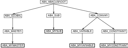
If we want to use ABACUS for a new application we have to derive problem specific classes from some base classes. Usually, only four base classes of ABACUS are involved: ABA_VARIABLE, ABA_CONSTRAINT, ABA_MASTER, and SUBPROBLEM. For some applications it is even possible that the classes ABA_VARIABLE and/or ABA_CONSTRAINT are not included in the derivation process if those concepts provided already by ABACUS are sufficient. By the definition of some pure virtual functions of the base classes in the derived classes and the redefinition of some virtual functions a problem specific algorithm can be composed. Figure 5.1 shows how the problem specific classes MYMASTER, MYSUB, MYVARIABLE, and MYCONSTRAINT are embedded in the inheritance graph of ABACUS.
Throughout this section we only use the default pool concept of ABACUS, i.e., we have one pool for static constraints, one pool for dynamically generated cutting planes, and one pool for variables. We will outline how an application specific pool concept can be implemented in Section 5.2.1.
The first step in the implementation of a new application is the analysis of its variable and constraint structure. We require at least one constraint class derived from the class ABA_CONSTRAINT and at least one variable class derived from the class ABA_VARIABLE. The used variable and constraint classes have to match such that a row or a column of the constraint matrix of an LP-relaxation can be generated.
We derive from the class ABA_VARIABLE the class MYVARIABLE storing the attributes specific to the variables of our application, e.g., its number, or the tail and the head of the associated edge of a graph.
Then we derive the class MYCONSTRAINT from the class ABA_CONSTRAINT
class MYCONSTRAINT : public ABA_CONSTRAINT {
public: virtual double coeff(ABA_VARIABLE *v); }; |
The function ABA_CONSTRAINT::coeff(ABA_VARIABLE *v) is a pure virtual function. Hence, we define it in the class MYCONSTRAINT. It returns the coefficient of variable v in the constraint. Usually, we need in an implementation of the function coeff(ABA_VARIABLE *v) access to the application specific attributes of the variable v. Therefore, we have to cast v to a pointer to an object of the class MYVARIABLE for the computation of the coefficient of v. Such that this cast can be performed safely, the variables and constraints used within an application have to be compatible. If run time type information (RTTI) is supported on your system, these casts can be performed safely.
The function coeff() is used within the framework when the row format of a constraint is computed, e.g., when the linear program is set up, or a constraint is added to the linear program. When the column associated with a variable is generated, then the virtual member function coeff() of the class ABA_VARIABLE is used, which is in contrast to the function coeff() of the class ABA_CONSTRAINT not an abstract function:
double ABA_VARIABLE::coeff(ABA_CONSTRAINT *con)
{ return con->coeff(this); } |
This method of defining the coefficients of the constraint matrix via the constraints of the matrix originates from cutting plane algorithms. Whereas in a column generation algorithm we usually have a different view on the problem, i.e., the coefficients of the constraint matrix are defined with the help of the variables. In this case, it is appropriate to define the function MYCONSTRAINT::coeff(ABA_VARIABLE *v) analogously to the function ABA_VARIABLE::coeff(ABA_CONSTRAINT *v) and to define the the function MYVARIABLE::coeff(ABA_CONSTRAINT *v).
ABACUS provides two constraint/variable pairs in its application independent kernel. The most simple one is where each variable is identified by an integer number (class ABA_NUMVAR) and each constraint is represented by its nonzero coefficients and the corresponding number of the variables (class ABA_ROWCON). We use this constraint/variable pair for general mixed integer optimization problems.
The constraint/variable pair ABA_NUMCON/ABA_COLVAR is dual to the previous one. Here the constraints are given by an integer number, but we store the nonzero coefficients and the corresponding row numbers for each variable. Therefore, this constraint/variable pair is useful for column generation algorithms.
ABACUS is not restricted to a single constraint/variable pair within one application. There can be an arbitrary number of constraint and variable classes. It is only required that the coefficients of the constraint matrix can be safely computed for each constraint/variable pair.
There are two main reasons why we require a problem specific master of the optimization. The first reason is that we have to embed problem specific data members like the problem formulation. The second reason is the initialization of the first subproblem, i.e., the root node of the branch-and-bound tree has to be initialized with a subproblem of the class MYSUB. Therefore, a problem specific master has to be derived from the class ABA_MASTER:
class MYMASTER : public ABA_MASTER {};
|
Usually, the input data is read from a file by the constructor or they are specified by the arguments of the constructor.
From the constructor of the class MYMASTER the constructor of the base class ABA_MASTER must be called:
ABA_MASTER(const char *problemName, bool cutting, bool pricing,
ABA_OPTSENSE::SENSE optSense = ABA_OPTSENSE::Unknown, double eps = 1.0e-4, double machineEps = 1.0e-7, double infinity = 1.0e32); |
Whereas the first three arguments are mandatory, the other ones are optional.
| problemName | The name of the problem being solved. |
| cutting | If true, then cutting planes are generated. |
| pricing | If true, then inactive variables are priced out. |
| optSense | The sense of the optimization. |
| eps | A zero-tolerance used within all member functions of objects that have a pointer to this global object. |
| machineEps | Another zero tolerance to compare a value of a floating point variable with 0. This value is usually less than eps, because eps includes some “safety” tolerance, e.g., to test if a constraint is violated. |
| infinity | All floating point numbers greater than infinity are regarded as “infinitely big”. Please note that this value might be different from the value the LP-solver uses internally. You should make sure that the value used here is always greater than or equal to the value used by the solver. |
An optional argument of the constructor of the class ABA_MASTER is the sense of the optimization. For some problems (e.g., the binary cutting stock problem or the traveling salesman problem) the sense of the optimization is already known when this constructor is called. For other problems (e.g, the mixed integer optimization problem) the sense of the optimization is determined later when the input data is read in the constructor of the specific application. In this case, the sense of the optimization has to be initialized explicitly before the optimization is started with the function optimize().
The following example of a constructor for the class MYMASTER sets up the master for a branch-and-cut algorithm and initializes the optimization sense explicitly as it is read from the input file.
MYMASTER::MYMASTER(const char *problemName) :
ABA_MASTER(problemName, true, false), { // read the data from the file problemName if (/* problemName is a minimization problem*/) initializeOptSense(ABA_OPTSENSE::Min); else initializeOptSense(ABA_OPTSENSE::Max); } |
The constraints and variables that are not generated dynamically, e.g., the degree constraints of the traveling salesman problem or the constraints and variables of the problem formulation of a general mixed integer optimization problem, have to be set up and inserted in pools in a member function of the class MYMASTER. These initializations can be also performed in the constructor, but we recommend to use the virtual dummy function initializeOptimization() for this purpose, which is called after the optimization is started with the function optimize().
By default, ABACUS provides three different pools: one for variables and two for constraints. The first constraint pool stores the constraints that are not dynamically generated and with which the first LP-relaxation of the first subproblem is initialized. The second constraint pool is empty at the beginning and is filled up with dynamically generated cutting planes. In general, ABACUS provides a more flexible pool concept to which we will come back later, but for many applications the default pools are sufficient.
After the initial variables and constraints are generated they have to be inserted into the default pools by calling the function
virtual void initializePools(ABA_BUFFER<ABA_CONSTRAINT*> &constraints,
ABA_BUFFER<ABA_VARIABLE*> &variables, int varPoolSize, int cutPoolSize, bool dynamicCutPool = false); |
Here, constraints are the initial constraints, variables are the initial variables, varPoolSize is the initial size of the variable pool, and cutPoolSize is the initial size of the cutting plane pool. The size of the variable pool is always dynamic, i.e., this pool is increased if required. By default, the size of the cutting plane pool is fixed, but it becomes dynamic if the argument dynamicCutPool is true.
There is second version of the function |initializePools()| that allows the insertion of an initial set of cutting planes into the cut pool.
The function initializeOptimization() can be also used to determine a feasible solution by a heuristic such that the primal bound can be initialized.
Hence, the function initializeOptimization() could look as follows under the assumption that the functions nVar() and nCon() are defined in the class MYMASTER and return the number of variables and the number of the constraints, respectively. In the example we initialize the size of the cut pool with 2*nCon(). As the arguments of the constructors of the classes MYVARIABLE and MYCONSTRAINT are problem specific we replace them by “…”.
After the pools are set up the primal bound is initialized with the value of a feasible solution returned by the function myHeuristic(). While the initialization of the pools is mandatory the initialization of the primal bound is optional.
void MYMASTER::initializeOptimization()
{ ABA_BUFFER<ABA_VARIABLE*> variables(this, nVar()); for (int i = 0; i < nVar(); i++) variables.push(new MYVARIABLE(...)); ABA_BUFFER<ABA_CONSTRAINT*> constraints(this, nCon()); for (i = 0; i < nCon(); i++) constraints.push(new MYCONSTRAINT(...)); initializePools(constraints, variables, nVar(), 2*nCon()); primalBound(myHeuristic()); } |
The root of the branch-and-bound tree has to be initialized with an object of the problem specific subproblem class MYSUB, which is derived from the class ABA_SUB. This initialization must be performed by a definition of the pure virtual function firstSub(), which returns a pointer to the first subproblem. In the following example we assume that the constructor of the class MYSUB for the root node of the enumeration tree has only a pointer to the associated master as argument.
ABA_SUB *MYMASTER::firstSub()
{ return new MYSUB(this); } |
Finally, we have to derive a problem specific subproblem from the class ABA_SUB:
class MYSUB : public ABA_SUB {};
|
Besides the constructors only two pure virtual functions of the base class ABA_SUB have to be defined, which check if a solution of the LP-relaxation is a feasible solution of the mixed integer optimization problem, and generate the sons after a branching step, respectively. Moreover, the main functionality of the problem specific subproblem is to enhance the branch-and-bound algorithm with dynamic variable and constraint generation and sophisticated primal heuristics.
The class ABA_SUB has two different constructors: one for the root node of the optimization and one for all other subproblems of the optimization. This differentiation is required as the constraint and variable set of the root node can be initialized explicitly, whereas for the other nodes this data is copied from the father node and possibly modified by a branching rule. Therefore, we also have to implement these two constructors for the class MYSUB.
The root node constructor for the class ABA_SUB must be called from the root node constructor of the class MYSUB.
ABA_SUB(ABA_MASTER *master,
double conRes, double varRes, double nnzRes, bool relativeRes = true, ABA_BUFFER<ABA_POOLSLOT<ABA_CONSTRAINT, ABA_VARIABLE> *> *constraints = 0, ABA_BUFFER<ABA_POOLSLOT<ABA_VARIABLE, ABA_CONSTRAINT> *> *variables = 0); |
| master | A pointer to the corresponding master of the optimization. |
| conRes | The additional memory allocated for constraints. |
| varRes | The additional memory allocated for variables. |
| nnzRes | The additional memory allocated for nonzero elements of the constraint matrix. |
| relativeRes | If this argument is true, then reserve space for variables, constraints, and nonzeros of the previous three arguments is given in percent of the original numbers. Otherwise, the numbers are interpreted as absolute values (casted to integer). |
| constraints | The pool slots of the initial constraints. If the value is 0, then all constraints of the default constraint pool are taken. |
| variables | The pool slots of the initial variables. If the value is 0, then all variables of the default variable pool are taken. |
The values of the arguments conRes, varRes, and nnzRes should only be good estimations. An underestimation does not cause a run time error, because space is reallocated internally as required. However, many reallocations decrease the performance. An overestimation only wastes memory.
In the following implementation of a constructor for the root node we do not specify additional memory for variables, because we suppose that no variables are generated dynamically. We accept the default settings of the last three arguments, as this is normally a good choice for many applications.
MYSUB::MYSUB(MYMASTER *master) :
ABA_SUB(master, 50.0, 0.0, 100.0) { } |
While there are some alternatives for the implementation of the root node for the application, the constructor of non-root nodes has usually the same form for all applications, but might be augmented with some problem specific initializations.
MYSUB::MYSUB(ABA_MASTER *master, ABA_SUB *father, ABA_BRANCHRULE *branchRule) :
ABA_SUB(master, father, branchRule) {} |
| master | A pointer to the corresponding master of the optimization. |
| father | A pointer to the father in the enumeration tree. |
| branchRule | The rule defining the subspace of the solution space associated with this node. More information about branching rules can be found in Section 5.2.7. As long as you are using only the default branching on variables you do not have to know anything about the class ABA_BRANCHRULE. |
The root node constructor for the class MYSUB has to be called from the function firstSub() of the class MYMASTER. The constructor for non-root nodes has to be called in the function generateSon() of the class MYSUB.
After the LP-relaxation is solved we have to check if its optimum solution is a feasible solution of our optimization problem. Therefore, we have to define the pure virtual function feasible() in the class MYSUB, which should return true if the LP-solution is a feasible solution of the optimization problem, and false otherwise:
bool MYSUB::feasible()
{} |
If all constraints of the integer programming formulation are present in the LP-relaxation, then the LP-solution is feasible if all discrete variables have integer values. This check can be performed by calling the member function integerFeasible() of the base class ABA_SUB:
bool MYSUB::feasible()
{ return integerFeasible(); } |
If the LP-solution is feasible and its value is better than the primal bound, then ABACUS automatically updates the primal bound. However, the update of the solution itself is problem specific, i.e., this update has to be performed within the function feasible().
Like the pure virtual function firstSub() of the class ABA_MASTER, which generates the root node of the branch-and-bound tree, we need a function generating a son of a subproblem. This function is required as the nodes of the branch-and-bound tree have to be identified with a problem specific subproblem of the class MYSUB. This is performed by the pure virtual function generateSon(), which calls the constructor for a non-root node of the class MYSUB and returns a pointer to the newly generated subproblem. If the constructor for non-root nodes of the class MYSUB has the same arguments as the corresponding constructor of the base class ABA_SUB, then the function generateSon() can have the following form:
ABA_SUB *MYSUB::generateSon(ABA_BRANCHRULE *rule)
{ return new MYSUB(master_, this, rule); } |
This function is automatically called during a branching process. If the already built-in branching strategies are used, we do not have to care about the generation of the branching rule rule. How other branching strategies can be implemented is presented in Section 5.2.7.
The two constructors, the function feasible(), and the function generateSon() must be implemented for the subproblem class of every application. As soon as these functions are available, a branch-and-bound algorithm can be performed. All other functions of the class MYSUB that we are going to explain now, are optional in order to improve the performance of the implementation.
Problem specific cutting planes can be generated by redefining the virtual dummy function separate(). In this case, also the argument cutting in the constructor of the class ABA_MASTER should receive the value true, otherwise the separation is skipped. The first step is the redefinition of the function separate() of the base class ABA_SUB.
int MYSUB::separate()
{ } |
The function separate() returns the number of generated constraints.
We distinguish between the separation from scratch and the separation from a constraint pool. Newly generated constraints have to be added by the function addCons() to the buffer of the class ABA_SUB, which returns the number of added constraints. Constraints generated in earlier iterations that have been become inactive in the meantime might be still contained in the cut pool. These constraints can be regenerated by calling the function constraintPoolSeparation(), which adds the constraints to the buffer without an explicit call of the function addCons().
A very simple separation strategy is implemented in the following example of the function separate(). Only if the pool separation fails, we generate new cuts from scratch. The generated constraints are added with the function addCons() to the internal buffer, which has a limited size. The number of constraints that can still be added to this buffer is returned by the function addConBufferSpace(). The function mySeparate() performs here the application specific separation. If more cuts are added with the function addCons() than there is space in the internal buffer for cutting planes, then the redundant cuts are discarded. The function addCons() returns the number of actually added cuts.
int MYSUB::separate()
{ int nCuts = constraintPoolSeparation(); if (!nCuts) { ABA_BUFFER<ABA_CONSTRAINT*> newCuts(master_, addConBufferSpace()); nCuts = mySeparate(newCuts); if (nCuts) nCuts = addCons(newCuts); } return nCuts; } |
Note, ABACUS does not automatically check if the added constraints are really violated. Adding only non-violated constraints, can cause an infinite loop in the cutting plane algorithm, which is only left if the tailing off control is turned on (see Section 5.2.26).
While constraints added with the function addCons() are usually allocated by the user, they are deleted by ABACUS. They must not be deleted by the user (see Section 5.2.13).
If not all constraints of the integer programming formulation are active, and all discrete variables have integer values, then the solution of a separation problem might be required to check the feasibility of the LP-solution. In order to avoid a redundant call of the same separation algorithm later in the function separate(), constraints can be added already here by the function addCons().
In the following example of the function feasible() the separation is even performed if there are discrete variables with fractional values such that the separation routine does not have to be called a second time in the function separate().
bool MYSUB::feasible()
{ bool feasible; if (integerFeasible()) feasible = true; else feasible = false; ABA_BUFFER<ABA_CONSTRAINT*> newCuts(master_, addConBufferSpace()); int nSep = mySeparate(newCuts); if (nSep) { feasible = false; addCons(newCuts); } return feasible; } |
The dynamic generation of variables is performed very similarly to the separation of cutting planes. Here, the virtual function pricing() has to be redefined and the argument pricing in the constructor of the class ABA_MASTER should receive the value true, otherwise the pricing is skipped.
We illustrate the redefinition of the function pricing() by an example that is an analogon to the example given for the function separate().
int MYSUB::pricing()
{ int nNewVars = variablePoolSeparation(); if (!nNewVars) { ABA_BUFFER<ABA_VARIABLE*> newVariables(master_, addVarBufferSpace()); nNewVars = myPricing(newVariables); if (nNewVars) nNewVars = addVars(newVariables); } return nNewVars; } |
While variables added with the function addVars() are usually allocated by the user, they are deleted by ABACUS. They must not be deleted by the user (see Section 5.2.13).
After the LP-relaxation has been solved in the subproblem optimization the virtual function improve() is called. Again, the default implementation does nothing but in a redefinition in the derived class MYSUB application specific primal heuristics can be inserted:
int MYSUB::improve(double &primalValue)
{ } |
If a better feasible solution is found its value has to be stored in primalValue and the function should return 1, otherwise it should return 0. In this case, the value of the primal bound is updated by ABACUS, whereas the solution itself has to be updated within the function improve() as already explained for the function feasible().
It is also possible to update the primal bound already within the function improve() if this is more convenient to reduce internal bookkeeping. In the following example we apply the two problem specific heuristics myFirstHeuristic() and mySecondHeuristic(). After each heuristic we check if the value of the solution is better than the best known one with the function call master_->betterPrimal(value). If this function returns true we update the value of the best known feasible solution by calling the function master_->primalBound().
int MYSUB::improve(double &primalValue)
{ int status = 0; double value; myFirstHeuristic(value); if (master_->betterPrimal(value)) { master_->primalBound(value); primalValue = value; status = 1; } mySecondHeuristic(value); if (master_->betterPrimal(value)) { master_->primalBound(value); primalValue = value; status = 1; } return status; } |
For a complete description of all members of the class ABA_SUB we refer to the documentation in the reference manual. However, in most applications only a limited number of data is required for the implementation of problem specific functions, like separation or pricing functions. For simplification we want to state some of these members here:
| int nCon() const; | returns the number of active constraints. |
| int nVar() const; | returns the number of active variables. |
| ABA_VARIABLE *variable(int i); | returns a pointer to the i-th active variable. |
| ABA_CONSTRAINT *constraint(int i); | returns a pointer to the i-th active constraint. |
| double *xVal_; | an array storing the values of the variables after the linear program is solved. |
| double *yVal_ | an array storing the values of the dual variables after the linear program is solved. |
After the problem specific classes are defined as discussed in the previous sections, the optimization can be performed with the following main program. We suppose that the master of our new application has as only parameter the name of the input file.
#include ~mymaster.h~
int main(int argc, char **argv) { MYMASTER master(argv[1]); master.optimize(); return master.status(); } |